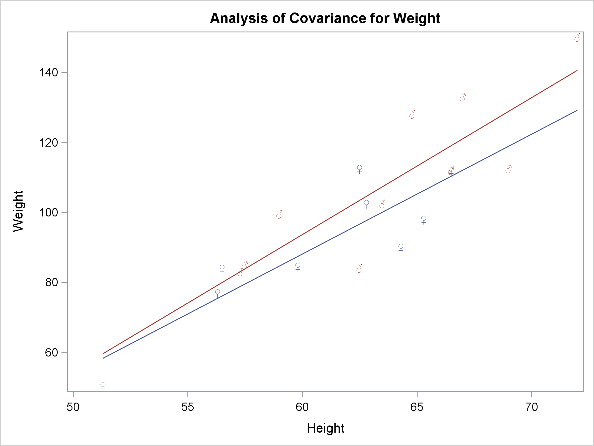
You can use Unicode to display special characters in SAS output including tables and graphs. When you control the graph yourself, as when you use PROC SGPLOT, you have complete control over specifying Unicode characters. When you are using analytical procedures, such as procedures in SAS/STAT, you are limited by the way that those procedures do things. That said, there are numerous ways that you can customize the default graphs. I have written about them extensively since the early days of ODS Graphics. This post is my latest installment. It shows how to get the Unicode characters where you want them, and it shows a number of other tricks along the way. First, let's see what the issue is. The following steps create a table of parameter estimates and a fit plot.
ods graphics on;
proc format;
   value $sexfmt 'M' = '(*ESC*){Unicode "2642"x}'
                 'F' = '(*ESC*){Unicode "2640"x}';
run;

proc glm data=sashelp.class;
   class sex;
   model weight = height | sex / solution;
   format sex $sexfmt.;
quit; |
My goal is to display female and male symbols instead of 'F' and 'M'. The table works just as you would expect.
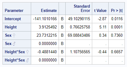
Then why does the graph legend look like this?
That was not what we were hoping for. To understand what happened, you need to understand a fundamental difference between how ODS tables and ODS Graphics process Unicode characters. When ODS is creating tables and it sees an escape sequence and a Unicode character in the value of a column, it substitutes the special character in the output. (This discussion does not apply to the LISTING destination.) When ODS is creating graphs and it sees an escape sequence and a Unicode character in the formatted value of a column, it substitutes the special character in the output. In other words, in ODS Graphics, you can only use Unicode with formats. You might argue, "But you used a format!" Yes I did, but PROC GLM did not send it to ODS Graphics. Most analytical procedures have SAS IO apply the formats and deliver character strings that contain the formatted values. PROC GLM and most other analytical procedures process character strings internally and not raw values. It will not matter if the CLASS variable is numeric or character, formatted or not, PROC GLM processes character strings that come from copying unformatted character variables or formatting other variables. This works fine until you get to a situation like this, which was not on anyone's mind when PROC GLM was first written over 40 years ago.
ODS Graphics needs to handle a large number of character variables and values. The developers made the decision to incur the extra overhead of Unicode only in limited situations, namely in values of variables that have user-defined formats. If we are going to see the Unicode characters, then we will need to modify the underlying data object to user formats. I will begin by enabling trace output so that I can see the object and template names.
ods trace on; proc glm data=sashelp.class; class sex; model weight = height | sex / solution; format sex $sexfmt.; quit; |
Output Added: ------------- Name: ANCOVAPlot Label: ANCOVA Plot Template: Stat.GLM.Graphics.ANCOVAPlot Path: GLM.ANOVA.Weight.ANCOVAPlot ------------- |
To recreate the graph outside the procedure, you need to capture the data object and dynamic variables. You can do that by running the following step.
ods document name=MyDoc (write); proc glm data=sashelp.class; ods output ancovaplot=ap; class sex; model weight = height | sex / solution; format sex $sexfmt.; quit; ods document close; |
The ODS DOCUMENT statements open and close the ODS document. You can get the dynamic variables from the document. The ODS OUTPUT statement captures in a data set the data object that underlies the graph.
The following step recreates the group variables to have the original 'F' and 'M' values and assigns the format.
data ap; set ap; if find(_group_fit, '40') then _group_fit = 'F'; if find(_group_fit, '42') then _group_fit = 'M'; if find(_group_obs, '40') then _group_obs = 'F'; if find(_group_obs, '42') then _group_obs = 'M'; format _group_obs _group_fit $sexfmt.; run; |
The following step lists the contents of the ODS document.
proc document name=MyDoc; list / levels=all; quit; |
The following step uses the path, copied and pasted from the previous step's output, to create an output data set that contains the names and values of all of the dynamic variables.
proc document name=MyDoc; ods output dynamics=dynamics; obdynam \GLM#1\ANOVA#1\Weight#1\ANCOVAPlot#1; quit; |
The following step uses CALL EXECUTE to generate a PROC SGRENDER step that recreates the graph. It uses the template name (as shown in the trace output) and the names and values of the dynamic variables.
data _null_;
   set dynamics(where=(label1 ne '___NOBS___')) end=eof;
   if _n_ = 1 then
      call execute('proc sgrender data=ap ' ||
                   'template=Stat.GLM.Graphics.ANCOVAPlot; dynamic');
   if cvalue1 ne ' ' then
      call execute(catx(' ', label1, '=',
                   ifc(n(nvalue1), cvalue1, quote(trim(cvalue1)))));
   if eof then call execute('; run;');
run; |
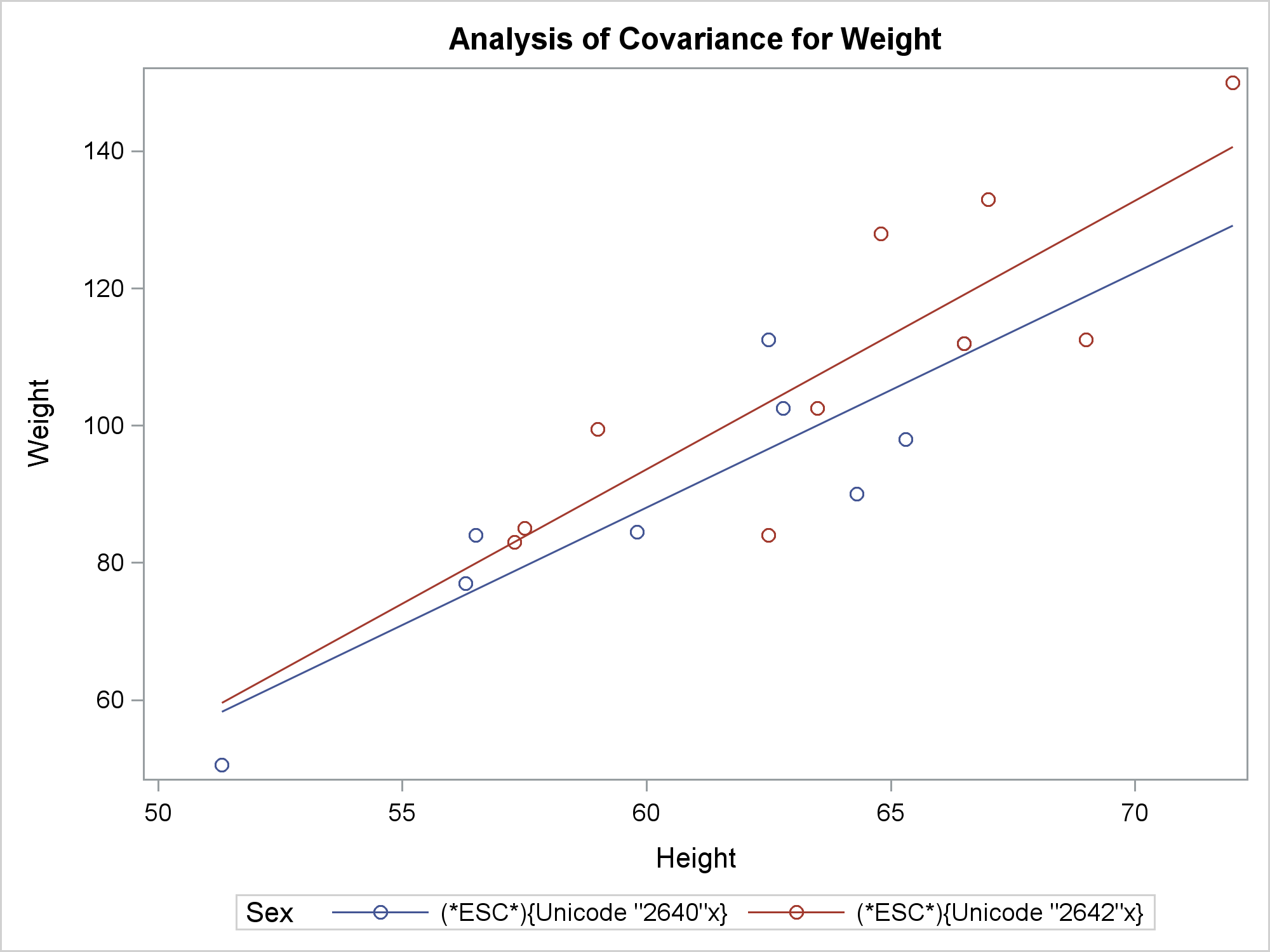
Unfortunately, we are not quite there. The legend now contains the right information, but it contains one extra entry for what it thinks is a missing group. To fix that, we will need to modify the graph template. Begin by examining the source code for the template. The first and second SOURCE statements show that there are a series of lines. The third SOURCE statement displays the actual template.
proc template; source Stat.GLM.Graphics.ANCOVAPlot; source Common.Zreg.Graphics.ANCOVAPlot; source Common.Zreg.Graphics.SLICEFITPlot; quit; |
This step writes the template to a file.
proc template; source Common.Zreg.Graphics.SLICEFITPlot / file='tpl.tpl'; quit; |
This step edits the template and submits it to SAS. It adds a PROC statement. While not necessary, it next changes the template name to the GLM template name. Finally, it adds the option INCLUDEMISSINGGROUP=FALSE to the SERIESPLOT statement. It took a bit of trial and error for me to figure out that that was what the template needed.
data _null_;
   infile 'tpl.tpl' end=eof;
   input;
   if _n_ = 1 then call execute('proc template;');

   _infile_ = tranwrd(_infile_, 'Common.Zreg.Graphics.SLICEFITPlot',
                                'Stat.GLM.Graphics.ANCOVAPlot');
   _infile_ = tranwrd(_infile_, 'primary=true',
                                'primary=true includemissinggroup=false');
   call execute(_infile_);
   if eof then call execute('run;');
run; |
I had to look at the template to see that the series plot was the primary plot. There are many ways I could have added the INCLUDEMISSINGGROUP=FALSE option to the SERIESPLOT statement. I chose to add it after the PRIMARY=TRUE option.
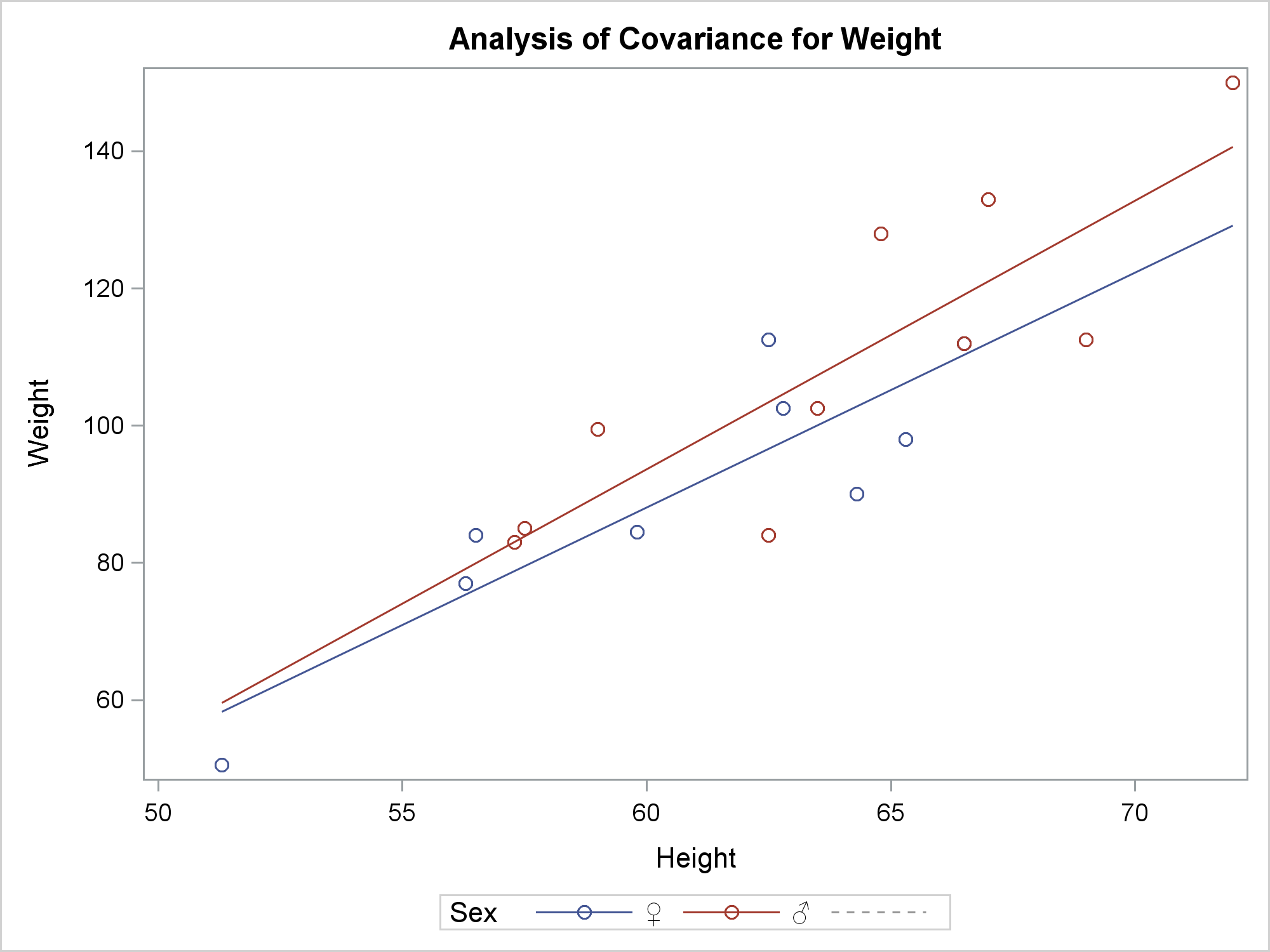
The last step uses the modified template to create the graph.
data _null_;
   set dynamics(where=(label1 ne '___NOBS___')) end=eof;
   if _n_ = 1 then
      call execute('proc sgrender data=ap ' ||
                   'template=Stat.GLM.Graphics.ANCOVAPlot; dynamic');
   if cvalue1 ne ' ' then
      call execute(catx(' ', label1, '=',
                   ifc(n(nvalue1), cvalue1, quote(trim(cvalue1)))));
   if eof then call execute('; run;');
run; |
You are no doubt wondering (as I did) why I needed to add INCLUDEMISSINGGROUP=FALSE to the template when it is used with PROC SGRENDER, but I did not need to add it when the graph is created with PROC GLM. The graph has two major components: a grouped scatter plot and a grouped series plot. There are 19 observations with nonmissing values that create the scatter plot. There are four observations with nonmissing values that create the series plot. There are two additional observations that are not plotted, but they ensure that the order of the CLASS values in the scatter plot match the order in the series plot. ODS Graphics in the context of PROC GLM has dynamic variables that contain the number of observations used. PROC SGRENDER does not have them. So PROC SGRENDER sees missing values in the series plot and adds them to the legend unless you specify INCLUDEMISSINGGROUP=FALSE.
There is one more difference. PROC SGRENDER prints a number of warnings; PROC GLM does not. When an analytical procedure runs, ODS Graphics assumes that it is using a general-purpose template that could be used for a variety of situations. Undefined dynamic variables and missing columns cause statements to silently drop out. In contrast, with PROC SGRENDER, ODS Graphics assumes that it is using an ad hoc user-written template, so all mismatches between what is specified and what is used are reported in the log.
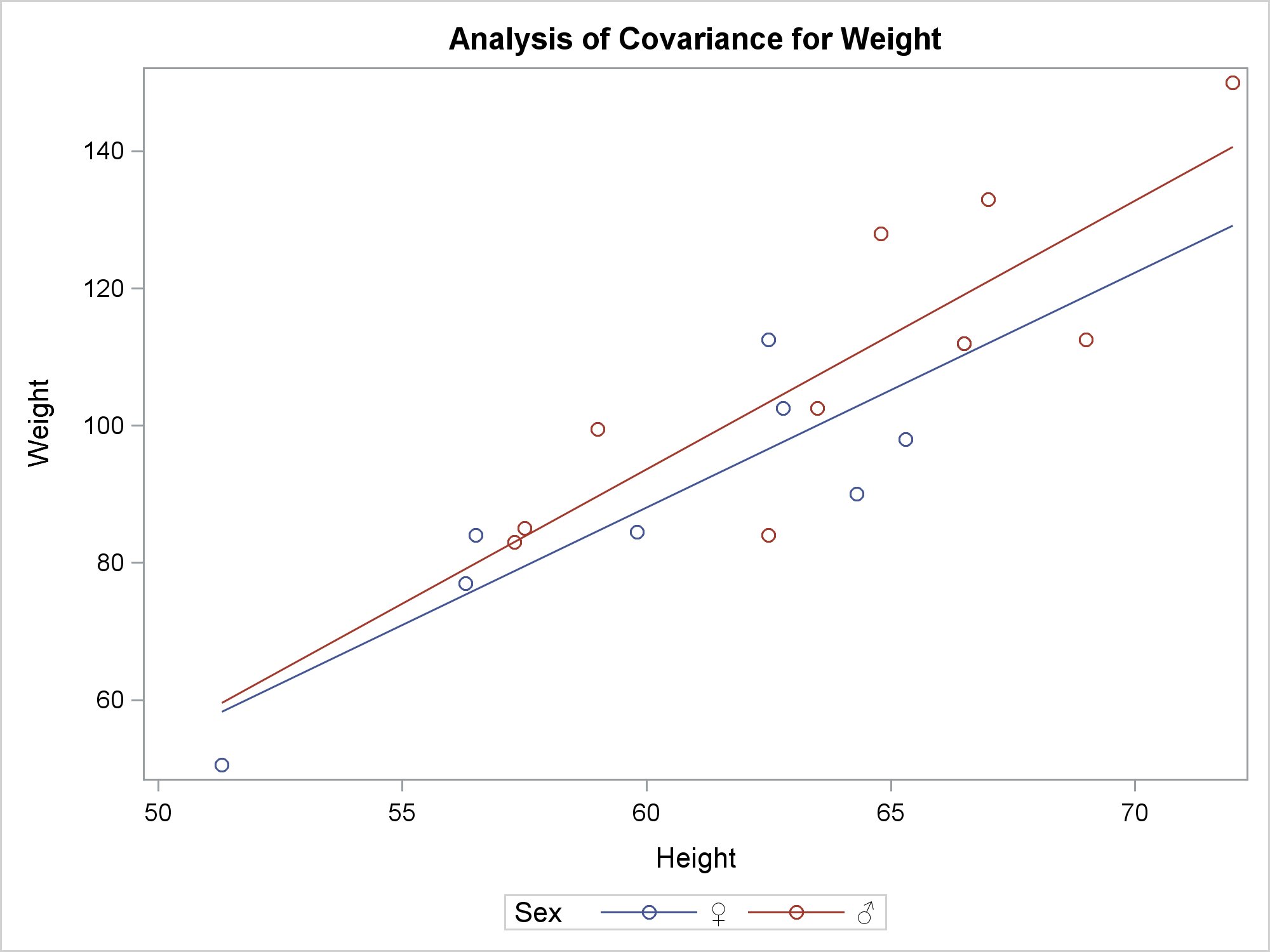
You could instead omit the legend and change the markers. The following step edits the template. It comments out the SCATTERPLOT statement and adds a TEXTPLOT statement before the ENDLAYOUT statement. The STRIP=TRUE option is critical here. The length of the formatted value is a bit ambiguous here. Is it the length of the escape and Unicode sequence or the length of a single character? The STRIP=TRUE option removes the trailing blanks before positioning the symbol so that ODS Graphics knows the length is a single character.
data _null_;
   infile 'tpl.tpl' end=eof;
   input;
   if _n_ = 1 then call execute('proc template;');

   _infile_ = tranwrd(_infile_, 'Common.Zreg.Graphics.SLICEFITPlot',
                                'Stat.GLM.Graphics.ANCOVAPlot');
   _infile_ = tranwrd(_infile_, 'primary=true',
                                'primary=true includemissinggroup=false');
   if find(_infile_, 'y=_Y_OBS') then
      _infile_ = tranwrd(_infile_, 'scatterplot', '*');
   if find(_infile_, 'endlayout;') then
      _infile_ = 'textplot y=_Y_OBS x=_XVAR_OBS text=_group_obs /
                  group=_GROUP_OBS strip=true;' || _infile_;
   call execute(_infile_);
   if eof then call execute('run;');
run; |
I cannot write code like this without first looking at the template that is stored in tpl.tpl. I wrote my code using the exact case that is in the template. I could instead use SAS functions to convert lines to lower or upper case and translate those.
The following step creates the graph.
data _null_;
   set dynamics(where=(label1 ne '___NOBS___')) end=eof;
   if _n_ = 1 then
      call execute('proc sgrender data=ap ' ||
                   'template=Stat.GLM.Graphics.ANCOVAPlot; dynamic');
   if cvalue1 ne ' ' then
      call execute(catx(' ', label1, '=',
                   ifc(n(nvalue1), cvalue1, quote(trim(cvalue1)))));
   if eof then call execute('; run;');
run; |
The last step deletes the modified template.
proc template; delete Stat.GLM.Graphics.ANCOVAPlot; quit; |
ODS Graphics gives you incredible flexibility to modify the graphs that come out of analytical procedures. Of course there are other ways you can do this. You can use the ODS output data set along with PROC SGPLOT. This would be easy for this example, but it might be harder for procedures that create a large number of dynamic variables. I like the approach of capturing the dynamic variables and programmatically modifying the template by using CALL EXECUTE. These methods enable you to create customized yet reproducible graphs.
For more on the ODS document and this type of graph customization, see my 2016 PharmaSUG paper. Rick Wicklin from the DO Loop blog provides a gentle introduction to advanced customization. I have also written about this topic extensively in other posts in Graphically Speaking.
As an exercise, what would be the easiest way to continue the customization and make the males blue and the females red or pink?


4 Comments
Very nice. I had encountered this just recently and was unable to find a solution, particularly with dynamic and macro vars. This will help for sure.
I had a similar issue with variable labels containing unicode characters. In the first example where I was using GTL to produce the graph the axis label which uses the var label did not work and I had to resort to adding the axis label to the template code. The other example using the same variable but with proc lifetest and ods graphics the label for the legend (in this case) was created as expected.
Not sure why this happened.
Pingback: How to fix common problems in output from ODS Graphics procedures - SAS Users
How to add header line in proc template for Forest Plot under Plotname, I am looking for correct option